The lowest in the world and falling? Explaining the movements of income inequality in Slovenia during the financial crisis
Andrej Srakar and Špela Zupan
Abstract
Gini coefficient in Slovenia is one of the lowest among the OECD countries and some recent findings show that in the last decade it further declined, despite the period of economic crisis that normally contributes to its increase. In our article we build upon existing empirical and theoretical studies on the topic that examined the levels of income inequality of Slovenia and other OECD countries in the past two decades and provide statistically grounded explanations for the fluctuations in Slovenian income inequality during the crisis by employing cointegration analysis. We calculate a series of inequality indices (e.g. Gini, Mehran, Piesch, Theil) for our sample of SORS 1993-2012 data on Slovenian employed population and derive the decomposition of Gini coefficient by the source of income. By using cointegration analysis, we examine the interrelationship of Gini coefficient and numerous other macroeconomic variables (e.g. GDP, unemployment levels, inflation). We show that several macroeconomic aggregates and social variables are related to inequality indices, but, interestingly, not including the levels of unemployment, which we use as a main explanation of the trend in the Slovenian income inequality in times of the financial crisis. In conclusion we reflect on the findings and their consequences for research and policy purposes.
During the last financial crisis and in its aftermath, the topic of social and income inequality, its determinants, and consequences gained a widespread popularity. Even though it has been the focus of research for many economists, Anthony Atkinson (2015), Joseph Stiglitz (2015a; 2015b), Steven Fazzari and Barry Cynamon (2013; 2015; 2016), Branko Milanović (2006), Thomas Piketty (2014) to mention just a few, the popularity outside the realms of academic world arrived with the publishing of the Thomas Piketty’s work The Capital in the 21st Century.
The above mentioned authors have been using different approaches to measure inequality and have identified different determinants of it, but the underlying conclusion for all of them has been that regardless of different historic, institutional and macroeconomic settings, inequality is one of the inherent causes of the economic crisis of capitalism.
Jan Rivkin (White, 2015) offers a brief systematic overview and trend development of the broadly specified main determinants of inequality, some of which are also included in our analysis.
Firstly, he identifies a decline in bargaining power of unions and lower social classes (also Podgursky, 1980), a determinant that Herzer (2016) analysed on the case of the USA and concluded that despite some evidence to the contrary (e.g. Partridge, Rickman & Levernier, 1996), a unilateral negative relationship between the intensity of the bargaining power of labour unions and income inequality exists due to the changes in distribution of income that follow a decrease in union presence.
Secondly, Rivkin points out class divergence as an issue of entire society and not only of the directly affected lower and middle class, and he explains it as a consequence of a disintegration of connection between companies and communities. His stance echoes the work of John Galbraith (1972; 1973), according to whom companies have a social responsibility to participate in education of workers, to participate in a development of public and common goods and to be more involved in a community they are set in, as that would alleviate some of the pressure that lower and middle class are facing and simultaneously benefit companies involved in the long run.
Thirdly, with the introduction of Ricardo's theory of comparative advantages in international trade, the effects of globalization on inequality decline were believed to be positive, as wages in developing countries would increase for unskilled labour and stagnate for skilled labour, thus closing/decreasing the gap (The Economist, 2014; IMF, 2007). This theory, however, has often been criticised (e.g. IMF, 2007; White, 2015) – overall impact of globalization turned out to be positive in absolute terms, as living standard of everyone, including the worst off individuals in developing countries, improved, but at the same time the income gap increased as well. IMF (2007) published a report arguing that the impact of globalization can be devided into two parts; while trade globalization contributes to a decrease, financial globalization contributes to an increase in income inequality, while their cummulative impact is still smaller than the one of technological advances. Authors also argue that liberalization of trade barriers and emphasis on wider education and credit availability would mitigate negative impacts of globalization.
Fourthly, different authors (e.g. IMF, 2007; Cardoso, Paes de Barros & Urani, 1995; OECD, 2012), recognize education and educational opportunities as important determinants of income inequality. Cardoso, Paes de Barros and Urani (1995) observed a significant explanatory value of education in their analysis of unemployment and inflation on the case of Brazil in the 1980s, but it was mostly limited to long-term trends in inequality, and education failed to explain short term oscilations of inequality. Stiglitz argues that inequality of opportunities in the US (and indirectly also income inequality) is higly dependent on the income and education of parents, and social mobility is significantly smaller that in the rest of developed world. Others (Hendel, Shapiro & Willen, 2004; OECD, 2012) argue that an increase in general educational level of a country, if achieved without corresponding policies that ensure more equal distribution of education opportunities, increases inequality as it moves a portion of disadvantaged individuals into a pool of educated ones, while simultaneously decreasing wages for unskilled labour and increasing skilled labour wages, hence increasing the income gap.
Fifthly, Milanovic and Van der Weide (2014) explain their findings through the mechanism of 'social separatism', in which they asssume that in a time of high inequality, the investments in public goods (e.g. education, health, infrastructure), which are essential for real income growth of lower and middle class, decline as rich prefer to keep the means for their own use, resulting in a further increase in income inequality. Anderson, de Renzion and Levy (2006) warn that the extent and strategy of an increase in investments in public goods and its impact on poverty levels are highly dependent on the country, »the structure of its economy and its initial physical public capital stock«.
Joseph Stiglitz (2015a; 2015b) argues that the previously dominant belief that inequality is caused by the imbalance of power between workers and capitalists should now be replaced with the analysis of the relationship between debt holders and equity holders. He also argues that the distribution of wealth is more unbalanced than the distribution of income, as one part of the population inherited their wealth (capitalists), while the rest accumulated it through savings (workers). General inequality increases with an increase of wealth to income ratio, and it is sensitive to changes in a ratio between r and g, which is also one of the premises that Piketty builds upon.
Piketty (2014) argues that even though r > g is an established assumption of most macroeconomic models, r (the net rate of return to capital) being larger than g (the growth rate of output) has potentially strong magnifying effect on inequality and causes an ‘inherent contradiction of capitalism’. As Srakar and Verbič (2015) synthesize, the contribution of Piketty’s analysis that mostly remains on a descriptive level is in its refusal to use mathematized economic models, while it still provides a systematic overview of the complexity of the issue. In light of rising disapproval of capitalism ensuing from the global economic crisis, his work also ignited a new wave of methodological pluralist and heterodox approaches to economics.
Anthony Atkinson (2015) and Fazzari and Cynamon (2013; 2015; 2016) argue that in order to decrease social inequality and with it correlated limited social mobility, policies, strengthening the progressive tax system, an implementation of the universal basic income, and widening of the social net should be implemented, governments should aim towards achieving higher employment, introducing carefull changes in fiscal and monetary policies, enforcing institutional changes that would facilitate wage growth and higher gender, and class equality in income distribution etc.
Despite being a very stern opponent of income and social inequality, Ghosh (2015) acknowledges that a certain level of inequality in society is beneficial as it incentivises individuals to innovate, work harder and strive for progress, however she emphasizes that there is a very thin line between acceptable level of inequality and prohibitive, harmful levels that perpetuate and increase social gap and decrease social mobility.
In the past two decades, a number of authors focused on the inequality related analysis of situation in Slovenia. Tomc and Pešec analysed socio-professional categories in Slovenia and discovered that differences between lower and middle category (class) are larger than between middle and top category, while differences between active and inactive research participants were also significant (as cited in Srakar & Verbič, 2015).
Dragoš and Leskošek examined the connection between social wealth and social inequality and identified three main types of simplifications; simplifications of social complexity, simplifications that are a result of ideological convictions and transitional losses of resources due to denationalisation and privatization, all of which affect analysed communities and behaviour of individuals (as cited in Srakar & Verbič, 2015).
Stanovnik (1997) discovered that characteristics of Slovenian economically worse off segments are converging towards characteristics of comparable socio-economic classes in other European countries, while studies done by Stanovnik and Verbič (2005; 2008; 2012; 2013; 2014) using empirical methodology also used by Piketty, explore the fluctuations of income inequality in Slovenia after it gained independence in 1991 (as cited in Srakar & Verbič, 2015). The authors discovered that controlling for the impact of initial years of transition, the increase in income inequality was neutralized through redistributive progressive taxation and through changes in institutional settings, while real income and consequently welfare were steadily increasing.
Penner, Kanjuo Mrčela, Bandelj and Petersen (2012) discovered that gender income inequality in private and public sector increased significantly between 1993 and 2007, but Leskovšek and Dragoš (2014) conclude, that Slovenia possesses capacities to cope with the issue (as cited in Srakar & Verbič, 2015). It is worth noting that despite an increase in income inequality, Slovenia presently remains one of the countries with the lowest Gini coefficient not only in OECD, but globally (OECD, 2013) and most recent findings (Srakar & Verbič, 2015) show, that income inequality in Slovenia in the past decade decreased despite economic crisis, prompting a question of what are the key determinants and causes behind such unusual decrease, a question that this paper attempts to answer (as cited in Srakar & Verbič, 2015).
In our article, we want to test the following main hypotheses: H1: Inequality in Slovenia in years 1993-2012 was strongly related to several macroeconomic variables, including level of GDP, inflation and general government expenditure. H2: Inequality in Slovenia in years 1993-2012 was strongly related to several social variables, including unemployment variables, social contributions and the level of older population. H3: The drops in Slovenian inequality in the years of the financial crisis were matched by movements of macroeconomic and/or social aggregates/variables.
In the following section we provide a brief description of the data and methodologies used, which include a series of inequality indices (e.g. Gini, Mehran, Piesch, Kakwani, Theil) and a decomposition of Gini coefficient by the source of income and gender. The third section contains the results of cointegration analysis and some basic findings related to the interrelationship of Gini coefficient and various macroeconomic variables examined, while in the final, fourth part key observations and conclusions are explained.
2. Methodology
The primary source of data was obtained by the Statistical Office of the Republic of Slovenia (SORS). Using Statistical Register of Employment (SRE), the annual (for the period 1993-2012) selection of the population of employees was done, who met the following two criteria: (a) full-time employed (which means that a person is working at least 36 hours per week) and (b) an employee of the same employer throughout the year. The data were obtained in tabular form for 14 income groups, depending on the employment sector (private and public), and gender (male, female), so that we have created for each income group and year four tables, which included broken sources of taxable income, as well as income tax and social security contributions. Tables covered the period from 1993 to 2012, which has enabled us to observe the developments in the economic crisis, which most previous studies did not cover.
Methodological analysis starts by calculating the indicators of income inequality. In doing so, the basic measure used is the Gini coefficient, which is the most commonly used measure of the uneven distribution of income and wealth. Gini coefficient is defined as the ratio on a scale between 0 and 1, the lower the ratio, the more equal the distribution, and the higher it is, the more uneven the distribution. The value 0 represents perfect equality (everyone having exactly the same revenue / property) while value 1 represents perfect inequality (all income / property is concentrated in only one individual).
In the analysis, we use the calculation of three related indicators of income inequality. Firstly, we use the Mehran and Piesch indices of inequality that have similar intepretations, but the weights used in the calculations are different. Mehran index is more sensitive to changes at the bottom of the income distribution, while Piesch is more sensitive to changes in the upper part of the income distribution. In addition to these three dimensions, we also use the Theil index of inequality, which is a measure of inequality based on the information theory, and was created by the econometrician Henri Theil in 1967. When calculating the value attributed to each event we evaluate the event which is highly likely as of low value, as the information on his occurence has not overly surprised us. Thus, the value of the information for the event to occur with a probability of 1 is equal to 0. Conversely, the occurrence of an unlikely event attributed to a high value (Kolenko, 2003).
Finally, we use cointegration analysis to evaluate the relationships between a set of chosen macroeconomic and social variables and our calculated inequality measures. We use Johansen trace test of cointegration. The common objective of cointegration tests is to determine if there exists a long-run relationship among all test variables (see e.g. Mencet, Firat & Sayin, 2006). All of these tests are designed to find the stationary linear combinations of vector time series, and in all of these tests a number of cointegrating factors must be determined. If the hypothesis is accepted, the error term (ut) is not stationary and this means that yt and xt series are not integrated. If the latter one is rejected, yt and xt are cointegrated. Note that since the unit root tests test the null hypothesis of a unit root, most cointegration tests test the null hypothesis of no cointegration.
On the other hand, sometimes regressing stationary data may eliminate the permanent components, leaving only the relations among the remaining stochastic components of the time series which may be pure noise, when what is of economic interest are actually the relations between the permanent components. Rudebusch (1992; 1993) demonstrates that standard unit root tests have low power against estimated trend stationary alternatives. In addition, Perron (1989) shows that standard unit root tests cannot always distinguish unit root from stationary processes that contain segmented or shifted trends. Nevertheless, some later research (Harvey, 1993; Engel and Morley, 2001; Morley, Nelson, et al., 2003; Morley, 2004; Sinclair, 2004) suggests that unobserved components models can provide a useful framework for representing economic time series which contain unit roots, including those that are cointegrated. These series can be modeled as containing an unobserved permanent component, representing the stochastic trend, and an unobserved transitory component, representing the stationary component of the series (for more see also Morley and Sinclair, 2005). This could be a solution for studying the relationships, discovered in our analysis in more detail in future, when the length of time series will allow for improved econometric modelling.
2. Results
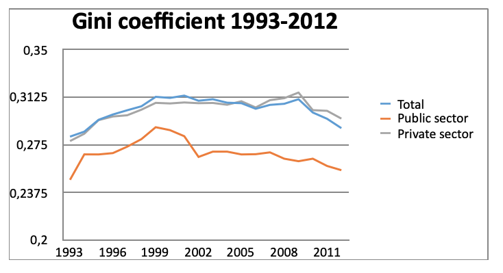
a. Basic indices Figure 1 shows the movement of the Gini coefficient for the entire sample in the period 1993-2012. After the initial substantial growth between 1993 and 1999, in the years 2000 to 2005, we see stagnation or even a small drop, then mild growth in the very beginning of the crisis (2007 and 2008), followed by a significant decline between 2009 and 2012. It is interesting that the first part of the fall (2009 and 2010) was led by the private sector, while the later decline in income inequality is expressed primarily in the public sector.
Figure 1: Gini coefficient, 1993-2012
Source: Own calculations.
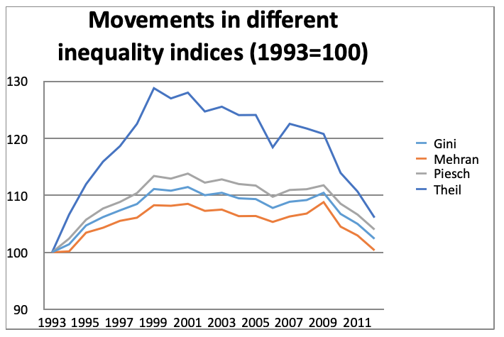
Figure 2 shows the correlation of movement with different dimensions of inequality. Comparison of Gini, Mehran and Piesch Inequality Index shows that Piesch index always has the highest value, while Mehran always the lowest value. Nevertheless, all three indexes speak the same story as an argument in favor of the thesis that the observed decline in income inequality has not been a consequence of specific developments either at the bottom or the top (such as a loss of better paid jobs, which would lead to a reduction in inequality at the expense of increased general poverty). The same story is shown also by the Theil index, but is expected to be far more sensitive to changes, although this sensitivity was not expressed in any way during the economic crisis. This shows us that for the rest of our research, the focus on Gini coefficient alone is sufficient, as it is a sufficiently reliable reflection of trends in income inequality during the observation period.
Figure 2: Movements in different inequality indices (1993=100)
Source: Own calculations.
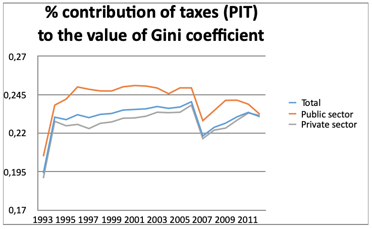
Here we used the decomposition of the Gini coefficient on the contribution of taxes, social security contributions and the net income to the level of inequality. Figure 3 shows the contribution of inequalities in taxes. We can see a relatively balanced picture until 2006, while after the Bajuk's tax reform after 2007, the disparity in taxes has fallen sharply, but later began to rise, although it still did not reach the previous levels. It is interesting to observe a decline in the contribution of taxes to the Gini coefficient in the years 2010-2012, which is specifically expressed in the public sector.
Figure 3: Contribution of taxes (Personal Income Tax) to the value of Gini coefficient
Source: Own calculations.
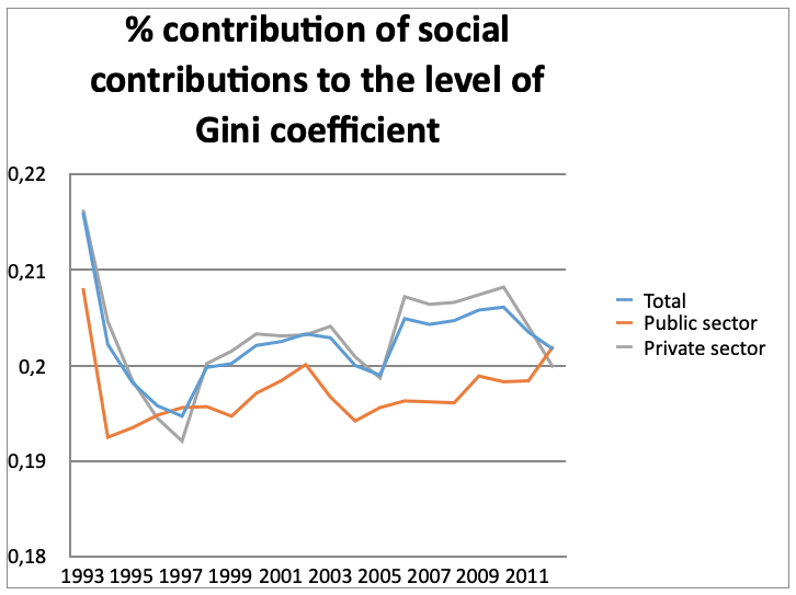
Figure 4 shows the dynamics of the contribution of social security contributions to the Gini coefficient. Particularly important are developments after 2007, when a considerable discrepancy between the public and private sectors has occured. In 2010, the contribution to overall income inequality in the private sector decreased significantly, while the trend in the public sector went in the opposite direction and has increased, particularly in 2012. The latter may be due to some initial layoffs after the introduction of the Law on Balancing Public Finances (ZUJF), but it could also be a consequence of a higher minimum wage, which resulted in the preservation of various forms of income for employees in the private sector. It is also important that the net effect of the two movements reduced total contribution from social contributions to the overall Gini coefficient.
Figure 4: Contribution of social contributions to the level of Gini coefficient
Source: Own calculations.
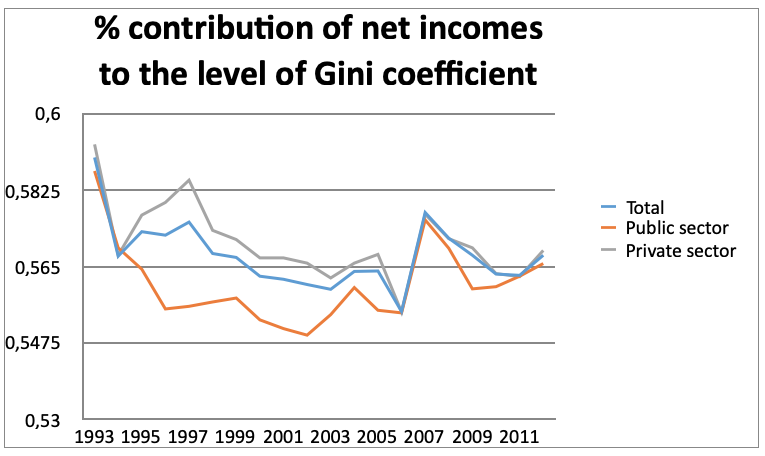
The most important and largest component of the Gini coefficient is the net income, where not exactly the same trends as previously can be observed during the economic crisis (see Figure 5). Firstly, the public and private sectors do not differ significantly. Secondly, in the years 2009 to 2012 there has been an increase in the impact of inequality in net income to the value of the Gini coefficient. Especially in the last two years, it has seen a stronger influence in the private sector, but it is difficult to conclude only on the basis of this, whether the observed trend of declining income inequality could be attributed to the public or private sector.
Figure 5: Contribution of net incomes to the level of Gini coefficient
Source: Own calculations.
b. Macroeconomic aggregates
In the second part of the analysis we look into relationships of a chosen set of macroeconomic variables and the previously calculated level of Gini coefficient. To this end we use 12 Slovenian macroeconomic aggregates, derived from the OECD database, namely:
Adjusted net national income per capita (constant 2005 US$)
Consumer price index (2010 = 100)
Final consumption expenditure (constant 2005 US$)
Foreign direct investment, net (BoP1, current US$)
GDP per capita (constant 2005 US$)
General government final consumption expenditure (% of GDP)
Gross national expenditure (% of GDP)
Gross savings (% of GDP)
Household final consumption expenditure (constant 2005 US$)
Interest payments (current LCU2)
Net domestic credit (current LCU)
Net foreign assets (current LCU)
All the variables have been shown to be of integration order I(2)3. In the figure below we firstly present co-movements in their values and the level of Gini index, that show the relationships of basic variables and the stationarity-adjusted second-differenced values.
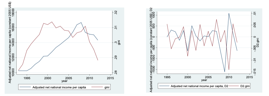
Figure 6 shows the co-movements between the Gini coefficient and adjusted net national income per capita. From the right side of the picture we cannot observe a significant cointegration – sometimes the levels of second differences are positively and sometimes negatively correlated. We will see later (see Table 1) that results of cointegration analysis confirm this observation.
Figure 6: Co-movements between adjusted net national income per capita and Gini index (Left: non-transformed variables; Right: second differences)
Source: Own calculations.
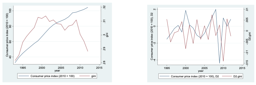
Figure 7 shows the relationship of inequality index and inflation. Again, no relationship can be observed. It has to be noted that in some of the results of the cointegration tests, presence of relationship between inequality and inflation has been confirmed, which would have to be better researched and reflected for future purposes.
Figure 7: Co-movements between consumer price index and Gini index (Left: non-transformed variables; Right: second differences)
Source: Own calculations.
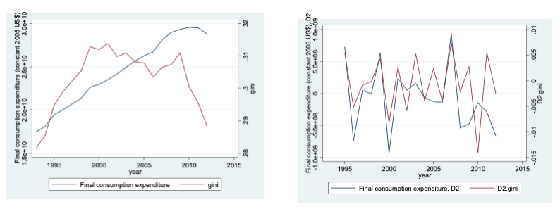
In Figure 8 we see the results of the relationship between final consumption expenditure and Gini index. As seen from Table 1, here cointegration can be confirmed, as seen from the right part of the figure, in particular for the years before the financial crisis, while during the financial crisis this relationship appears blurred and much weaker.
Figure 8: Co-movements between final consumption expenditure and Gini index (Left: non-transformed variables; Right: second differences)
Source: Own calculations.
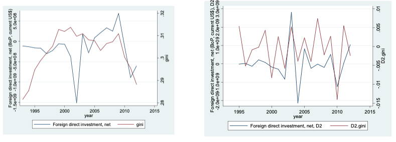
Also, the relationship between foreign direct investments and Gini index exists and is confirmed in Table 1. The relationship seems strong throughout the observed period, which can be seen in the right part of Figure 9.
Figure 9: Co-movements between foreign direct investment and Gini index (Left: non-transformed variables; Right: second differences)
Source: Own calculations.
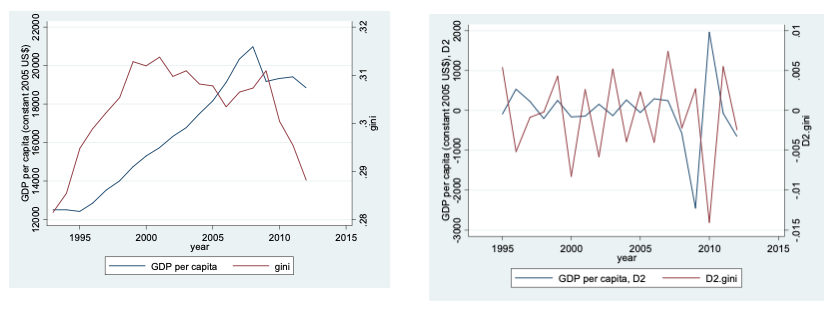
Interestingly, no particular relationship between GDP per capita and inequality could be confirmed for Slovenia (see Table 1). Nevertheless, the right part of Figure 10 shows a negative trend (in accordance with expectations – higher positive changes in the level of GDP are related to higher negative changes in inequality).
Figure 10: Co-movements between GDP per capita and Gini index (Left: non-transformed variables; Right: second differences)
Source: Own calculations.
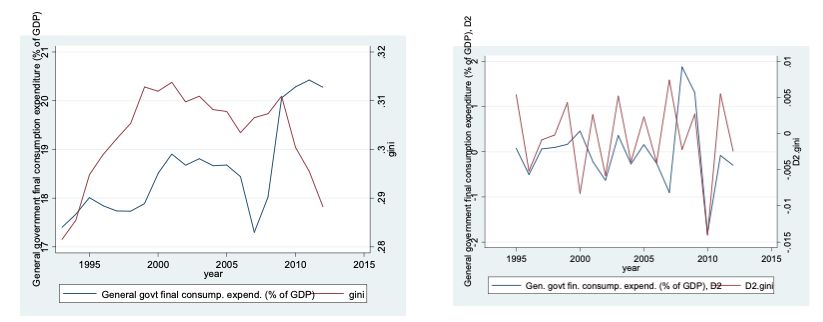
Figure 11 shows the relationship between general government consumption expenditure and the level of Gini index. There are some positive and negative co-movements, which result in the final no-cointegration relationship, as observed from Table 1.
Figure 11: Co-movements between general government consumption expenditure and Gini index (Left: non-transformed variables; Right: second differences)
Source: Own calculations.
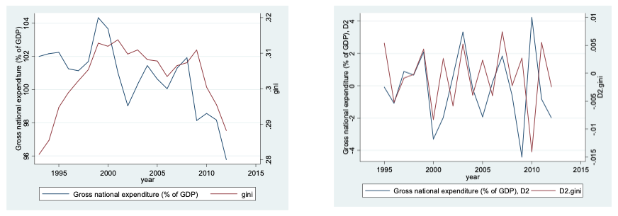
Also, we cannot confirm a relationship between gross national expenditure and the level of Gini index, which can again be seen from both the right part of the Figure 12 and the results in Table 1.
Figure 12: Co-movements between gross national expenditure and Gini index (Left:non-transformed variables; Right: seconddifferences)
Source: Own calculations.
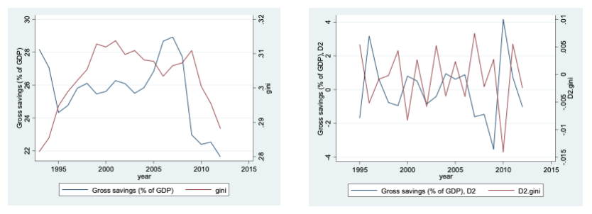
There is also no visible statistical relationship between the level of gross savings and Gini index. Again, several positive and negative co-movements can be seen in Figure 13 and results of Johansen's cointegration tests cannot confirm any relationship.
Figure 13: Co-movements between gross savings and Gini index (Left: non-transformed variables; Right: second differences)
Source: Own calculations.
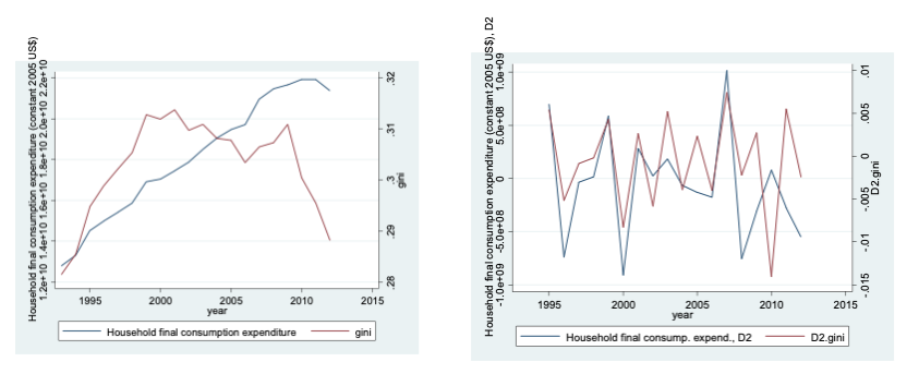
On the other hand, as Figure 14 shows, there is a relationship between household final consumption expenditure and Gini index, although seeming different for the period before and during the financial crisis (which is in accordance with the results of Figure 8, explained previously).
Figure 14: Co-movements between household final consumption expenditure and Gini index (Left: non-transformed variables; Right: second differences)
Source: Own calculations.
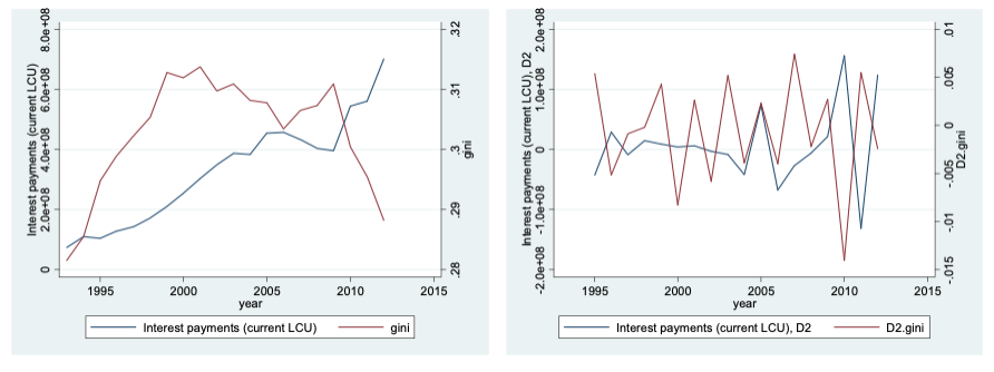
Interestingly, relationship between interest payments and Gini index can be confirmed, as seen from Table 1. This could be in particular related to the financial crisis, where the interest payments became particularly strong determinants of Slovenian macroeconomic condition. Also, from the right side of Figure 15 we can confirm different co-movements in times of the financial crisis and before it.
Figure 15: Co-movements between interest payments and Gini index (Left: non-transformed variables; Right: second differences)
Source: Own calculations.
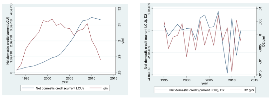
Also, as can be seen in Figure 16, relationship between net domestic credit and Gini index is confirmed from the results of Table 1. Again, the relationship seems to be conditioned by the financial crisis where the response has been exactly the opposite as before. Further tests of the presence of structural breaks would be needed to better explore this (and previously observed) different co-movements in times of the financial crisis.
Figure 16: Co-movements between net domestic credit and Gini index (Left: non-transformed variables; Right: second differences)
Source: Own calculations.
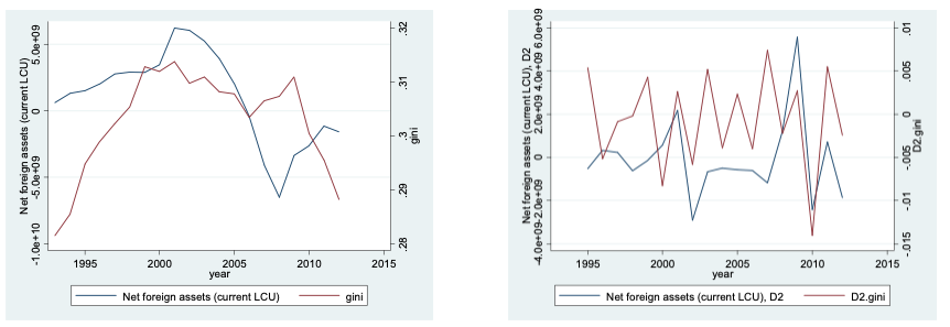
Finally, as shown in the Figure 17, net foreign assets are positively and strongly related to the level of Gini index, which is in accordance with Figure 9. Interestingly, foreign capital position seems very strongly and consistently related to the level of inequality, at least for Slovenia, which is particularly interesting considering the problems that Slovenia had with attracting foreign direct investments (being among the EU countries with their lowest share per capita). It is possible that the found relationship is either the consequence of a) problems in the modelling which didn't control sufficiently for small sample problems; b) we are modelling the stochastic component in two variables which seem particular to Slovenia, characterized by extremely low level of inequality on the one hand and very low level of FDI investments as well. It would be interesting in future to also model this stochastic component separately and explore its determinants and behaviour. Figure 17: Co-movements between net foreign assets and Gini index (Left: non-transformed variables; Right: second differences)
Source: Own calculations.
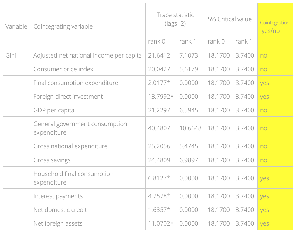
At the end, Table 1 shows the results of statistical tests. Six variables were confirmed as related to the level of inequality: final consumption expenditure and household final consumption expenditure; foreign direct investment and net foreign assets; interest payments; and net domestic credit. Clearly, the levels of domestic private consumption and the level of foreign investments are the most related to inequality in Slovenia, with GDP per capita and general government expenditure being far behind. Again, we note that this could be a consequence of modelling the stochastic part of the variables which should be separately modelled and explored better in future and could be the cause of some of the cointegration relationships. We also note that many variables that show cointegration properties are highly correlated (e.g. final consumption expenditure and household final consumption expenditure) which is in the nature of cointegration analysis, being a solution to the spurious correlation problem in the time series context (see e.g. Johansen, 2007). Nevertheless, the findings could have important consequences for understanding the movements of inequality not only in Slovenia but in other countries as well, if applied to other datasets. Table 1: Results of cointegration tests, macroeconomic aggregates, all variables are taken in first differences.
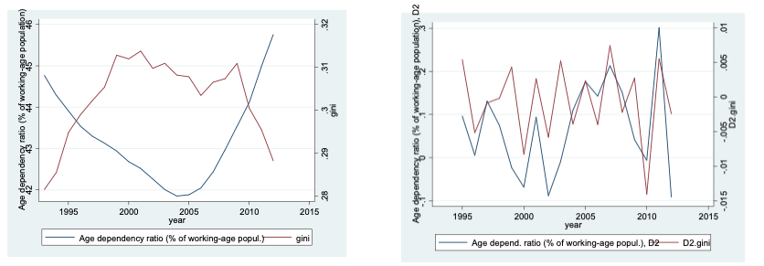
Note: Statistical significance: * – 5%. Source: Own calculations. Figure 18: Co-movements between age dependency ratio and Gini index (Left: non-transformed variables; Right: second differences)
Source: Own calculations.
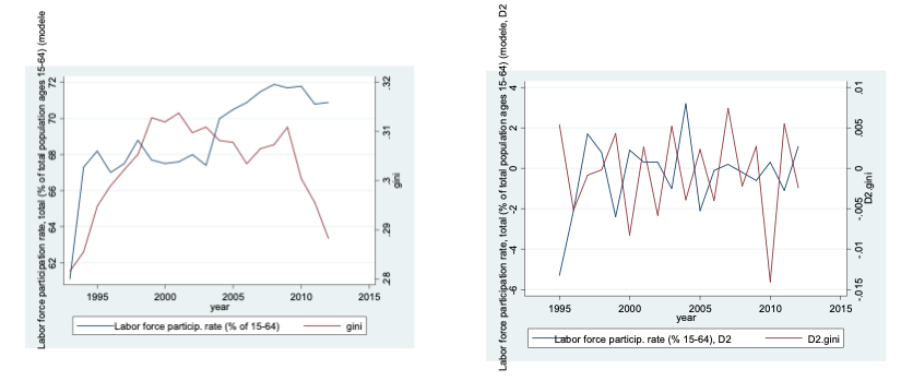
Labor force participation rate is not related to inequality, as shown in Figure 19. Interestingly and as will be seen later, employment levels were not related to inequality in Slovenia in years 1993-2012, which seems surprising and is perhaps a consequence of the choice of dataset which includes only employed persons (but this has to be tested further in future).
Figure 19: Co-movements between labor force participation rate and Gini index (Left: non-transformed variables; Right: second differences)
Source: Own calculations.
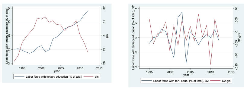
Also, the share of labor force with tertiary education is not related to the level of Gini index, although with some clear negative (and expected) co-movements, as shown in the left part of Figure 20. Figure 20: Co-movements between % labor force with tertiary education and Gini index (Left: non-transformed variables; Right: second differences)
Source: Own calculations.
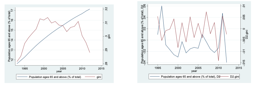
The size of older (65+) population is not related to inequality, which is visible from both results of Table 2 and left part of Figure 21. It is therefore interestingto see that age dependency ratio is related to inequalities, as opposed to the level of older population, which is not related to inequality, but that can probably be explained by the level of older population being a rather crude indicator, showing an almost linear rising trend for Slovenia in the period 1993-2012. Figure 21: Co-movements between population, aged 65 and above and Gini index (Left: non-transformed variables; Right: second differences)
Source: Own calculations.
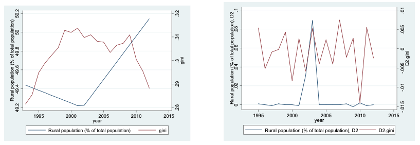
Interestingly, the share of rural population is strongly (Table 2) and negatively (left part of Figure 22) related to the level of inequality. This would be an indicator that Slovenian inequality among the employed workers is more related to the inequality among the urban population which is clearly seen in the left part of the Figure 22. Again, this would surely demand a better explanation that exceeds the depth of analysis of this paper, which only offers a robust conclusion. Figure 22: Co-movements between % of rural population and Gini index (Left: non-transformed variables; Right: second differences)
Source: Own calculations.
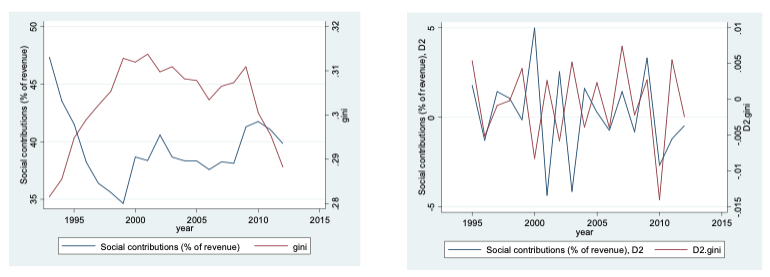
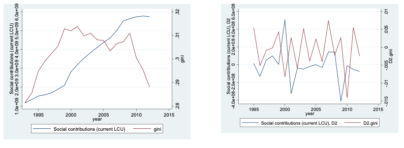
The share (in revenue composition; see Figure 23) and level of social contributions (Figure 24) is significantly related to inequality. This is hardly surprising, as social contributions were used in the calculation of the Gini index, and is presented here mainly as robustness verification and probably needs no further explanation.
Figure 23: Co-movements between social contributions as % of revenue and Gini index (Left: non-transformed variables; Right: second differences)
Source: Own calculations.
Figure 24: Co-movements between social contributions and Gini index (Left: non-transformed variables; Right: second differences)
Source: Own calculations.
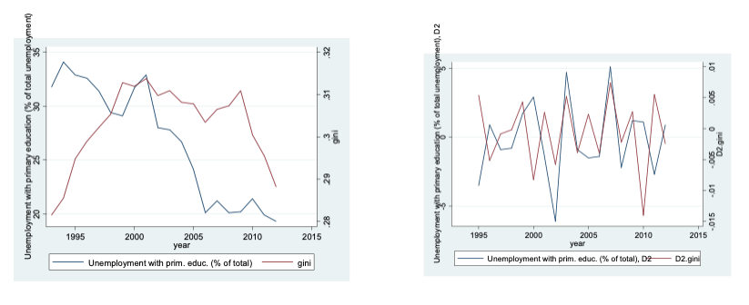
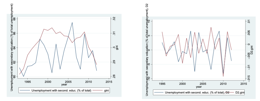
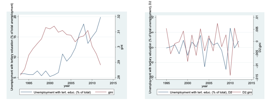
The final part of the analysis presents relationship between different employment variables and the level of inequality. Interestingly, no employment variable is in any sense related to the level of inequality. This holds, firstly, for the share of unemployed with both primary (Figure 25), secondary (Figure 26), as well as tertiary (Figure 27) education.
Figure 25: Co-movements between % of unemployed with primary education and Gini index (Left: non-transformed variables; Right: second differences)
Source: Own calculations.
Figure 26: Co-movements between % of unemployed with secondary education and Gini index (Left: non-transformed variables; Right: second differences)
Source: Own calculations.
Figure 27: Co-movements between % of unemployed with tertiary education and Gini index (Left: non-transformed variables; Right: second differences)
Source: Own calculations.
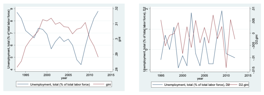
Next, this observation holds also for the total share of unemployed, although here the trace statistic is the closest to statistical significance (see Table 2). As can be seen from the Figure 28 (left part), in particular during the financial crisis, the level of unemployment was negatively related to inequality which could provide a clear explanation for the observed trend of falling (calculated) inequality during the financial crisis: in our sample we included only the employed persons and if we would include a different dataset, one that would include the active workforce in total, the results could completely change their sign and significance.
Figure 28: Co-movements between % of unemployed in total and Gini index (Left: non-transformed variables; Right: second differences)
Source: Own calculations.
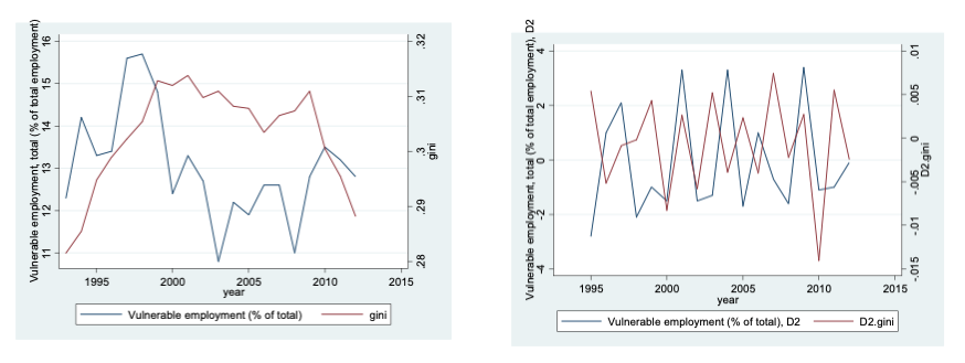
Also, no relationship to vulnerable employment could be observed (Figure 29), although here the visual results are more in accordance with expectations: less vulnerable employment appears related to also less inequality in general.
Figure 29: Co-movements between % of vulnerable employment and Gini index (Left: non-transformed variables; Right: second differences)
Source: Own calculations.
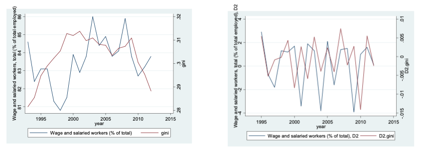
Finally, no visible relationship can be ascertained between the share of wage and salaried workers and Gini index, which is clearly confirmed from both Figure 30 and the results in Table 2.
Figure 30: Co-movements between % of wage and salaried workers and Gini index (Left: non-transformed variables; Right: second d ifferences)
Source: Own calculations.
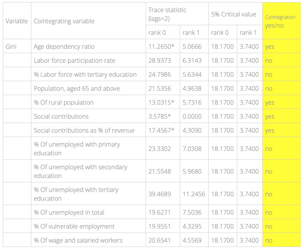
The results in Table 2 serve as a confirmation of the previous explanations. In total, four variables seem related to the level of inequality: age dependency ratio, share of rural population, and two variables related to social contributions. In particular, we were able to discern no statistically significant relationship to the employment variables, which is an interesting finding and could be a consequence of the used dataset.
Table 2: Results of cointegration tests, social variables, all variables are taken in first differences.
Note: Statistical significance: * – 5%. Source: Own calculations.
4. Discussion and conclusion
In conclusion, let's firstly shortly summarize the findings:
The level of inequality, as measured on the basis of used dataset, has been falling in times of the financial crisis, which seems in opposition ot the theories in the literature (in particular, Piketty 2014).
The differences could not be attributed to either the choice of the measure of inequality nor to the decomposition of the Gini index.
The level of inequality was shown to be related to several macroeconomic aggregates, in particular: final consumption expenditure and household final consumption expenditure; foreign direct investment and net foreign assets; interest payments; and net domestic credit.
Clearly, the levels of domestic private consumption and the level of foreign investments are the most related to inequality in Slovenia, with GDP per capita and general government expenditure being far behind. This could have important consequences for understanding the movements of inequality in Slovenia and wider, if applied to other datasets.
As for the relationship to the »social« variables, in total, four variables seem related to the level of inequality: age dependency ratio, share of rural population, and two variables related to social contributions. In particular, we were able to discern no statistically significant relationship to the employment variables, which is an interesting finding and could be a consequence of the used dataset.
There seem several different explanations for the observed trend of dropping inequality during the financial crisis in Slovenia. The main one, appearing from our analysis, seems related to the dataset: as we include only the employed people we neglect the influence of significantly raised unemployment in Slovenia. Another explanation is related to the raise in minimal wage, which would clearly have to have a strong effect on the level of inequality, as shown in the literature. Finally, institutional reasons show that the specific character of Slovenian institutional environment could be another reason for the observed trend. Nevertheless, all the above explanations have to be further explored and tested in the analysis. Our analysis, neveretheless, provided an important step forward in exploring not just inequality in Slovenia but also in a broader sense and we provided, to our knowledge, a novel methodology to study inequality, which should be developed in future research to get a significantly better insight into the determinants of economic and social inequality in general.
1 Balance of payments.
2 Local Currency Unit.
3 The results were derived using basic stationarity tests (ADF, KPSS) and are not reported here.
Cardoso, E., Paes de Barros, R., & Urani, A. (1995). Inflation and Unemployment as Determinants of Inequality in Brazil: The 1980s. In Reform, Recovery, and Growth: Latin America and the Middle East, eds. R. Dornbusch and S. Edwards, Chicago: University of Chicago Press, pp. 151 – 176. Retrieved from http://www.nber.org/chapters/c7655.pdf (accessed July 20th, 2016).
Cynamon, B. Z. & Fazzari, S. M. (2016). Inequality, the Great Recession and slow recovery. Camb. J. Econ., (2016), 40 (2): 373-399, doi: 10.1093/cje/bev016.
Dragoš, S., & Leskošek, V. (2003). Družbena neenakost in socialni kapital. Ljubljana: Mirovni inštitut, Inštitut za sodobne družbene in politične študije.
Engel, C. & Morley, J.C. (2001). The Adjustment of Prices and the Adjustment of the Exchange Rate. NBER Working Paper Series: Working Paper 8550.
Galbraith, J. K. (1972). The Emerging Public Corporation. Business and Society Review, 1: 54-56, reprinted in Steiner & Steiner, (eds) 1977: 2530-533.
Galbraith, J. K. (1973). On the Economic image of Corporate Enterprise in Nader & Green (eds) (1973)
Ghosh, J. (2015). Social Mobility in Subsaharan Africa, Latin America and Asia. International Development Economics Associates lecture. Retrieved from http://www.ideaswebsite.org/articles.php?aid=2303 (accessed July 8th, 2016).
Harvey, A. C. (1993). Time Series Models. Cambridge, MA, MIT Press.
Hendel, I., Shapiro, J. & Willen, P. (2005). Educational opportunity and income inequality, Journal of Public Economics, Elsevier, vol. 89(5-6), 841-870.
Herzer, D. (2016). Unions and Income Inequality – A panel cointegration and causality analysis for the United States. Economic Development Quarterly, August 2016, vol. 30, no. 3, 267-274.
Johansen, S. (2007). Correlation, Regression, and Cointegration of Nonstationary Economic Time Series (November 6, 2007). CREATES Research Paper No. 2007-35. Available at SSRN: https://ssrn.com/abstract=1150541 or http://dx.doi.org/10.2139/ssrn.1150541 (accessed November 15th, 2016).
Kolenko, A. (2003). Dekompozicija mer neenakosti. Bachelor Thesis, Ljubljana: Faculty of Economics.
Leskošek, V., & Dragoš, S. (2014). Social Inequality and Poverty in Slovenia – Policies and Consequences, Družboslovne razprave, XXX (2014), 76: 39–53.
Mencet, M.N., Firat, M.Z., Sayin, C. (2006). Cointegration analysis of wine export prices for France, Greece and Turkey. Paper prepared for presentation at the 98 th EAAE Seminar ‘Marketing Dynamics within the Global Trading System: New Perspectives’, Chania, Crete, Greece as in: 29 June – 2 July, 2006.
Milanović, B. (2006). Global income inequality: what it is and why it matters. Policy Research Working Paper Series 3865, The World Bank. Retrieved from http://www.un.org/esa/desa/papers/2006/wp26_2006.pdf (accessed July 20th, 2016).
Milanovic, B., & Van der Weide, R. (2014). Inequality is bad for income growth of the poor (but not for that of the rich).Retrieved from http://www.voxeu.org/article/good-rich-bad-poor (accessed July 20th, 2016).
Morley, J. C. (2004). The Slow Adjustment of Aggregate Consumption to Permanent Income. Working Paper, Washington University.
Morley, J. C., Nelson, C. R. et al. (2003). Why Are the Beveridge-Nelson and Unobserved-Components Decompositions of GDP So Different? The Review of Economics and Statistics 85(2): 235-243.
Morley, J. & Sinclair, T. M. (2005). Testing for Stationarity and Cointegration in an Unobserved Components Framework. Computing in Economics and Finance 2005 451, Society for Computational Economics.
OECD. (2013). Crisis squeezes income and puts pressure on inequality and poverty. Paris: OECD. Retrieved from http://www.oecd.org/els/soc/OECD2013-Inequality-and-Poverty-8p.pdf, 19. 12. 2014 & 22.06.2016. (accessed July 15th, 2016).
Partridge, M. D., Rickman, D. S., & Levernier, W. (1996). Trends in U.S. income inequality: Evidence from a panel of states. The Quarterly Review of Economics and Finance, Volume 36, Issue 1, Spring 1996, 17-37.
Penner, Andrew M., Kanjuo Mrčela, A., Bandelj, N. & Petersen, T. (2012). Neenakost po spolu v Sloveniji od 1993 do 2007: razlike v plačah v perspektivi ekonomske sociologije, Teorija in praksa, let. 49, 6/2012, 854–877.
Perron, P. (1989). The Great Crash, the Oil Price Shock, and the Unit Root Hypothesis. Econometrica 57: 1361-1401.
Piketty, T. (2014). Capital in the Twenty-first Century, Cambridge and London: Harvard University Press.
Rudebusch, G. D. (1992). Trends and Random Walks in Macroeconomic Time Series: A Re-Examination. International Economic Review 33: 661-680.
Rudebusch, G. D. (1993). The Uncertain Unit Root in Real GNP. The American Economic Review 83: 264-272.
Sinclair, T. M. (2004). Permanent and Transitory Movements in Output and Unemployment: Okun's Law Persists. Washington University Working Paper. St. Louis.
Srakar, A., & Verbič, M. (2015). Dohodkovna neenakost v Sloveniji in gospodarska kriza. Teorija in praksa, 52(3): 538-553.
Stanovnik, T. (1997). Revščina in marginalizacija prebivalstva v Sloveniji. Družboslovne razprave, Vol. XIII (1997) 24/25.
Stanovnik, T., & Verbič, M. (2005). Wage and Income Inequality in Slovenia, 1993–2002. Post-Communist Economies, 17(3): 381–397.
Stanovnik, T., & Verbič, M. (2008). Analiza neenakosti v porazdelitvi dohodkov zaposlenih v Sloveniji v obdobju 1991–2005. IB Revija, 42(3–4): 30–42.
Stanovnik, T., & Verbič, M. (2012). Porazdelitev plač in dohodkov zaposlenih v Sloveniji v obdobju 1991–2009. IB Revija, 46(1): 57–70.
Stanovnik, T., & Verbič, M.(2013). Earnings Inequality and Tax Progressivity in Slovenia, 1991–2009. Acta Oeconomica, 63(4): 405–421.
Stanovnik, T., & Verbič, M. (2014). Personal Income Tax Reforms and Tax Progressivity in Slovenia, 1991–2012. Financial Theory and Practice, IPF Zagreb, 38(4): 441–463.
Stiglitz, J. E., (2015a). Lecture on the Distribution of Income and Wealth Among Individuals: Theoretical Perspectives. Institute for New Economic Thinking.
Stiglitz, J. E., (2015b). New Theoretical Perspectives on the Distribution of Income and Wealth among Individuals: Part III: Life Cycle Savings vs. Inherited Savings. Institute for New Economic Thinking.