On Price Normalization and Choice of Techniques in Ricardo΄s TheoryAbstract
Ricardo’s corn model was the first model that made the unambiguous rank, comparison and choice of techniques, with respect to their profitability, possible. The problem of choosing techniques will be mathematically formulized and a solution based on the corn model will be provided. For those, who are familiar with the problem of price determination, it is well known that it is impossible to determine prices, for a given nominal wage, without determining profit rate first. From the price determination system, a relation between nominal wage and profit rate can be obtained, known as the w-r relation. To obtain the w-r relation, and fully determine prices, the price of a single commodity, or of a basket of commodities should be exogenously determined. The w-r relation as it will be shown in this paper is sensitive in the above arbitrary price determination. This vicious cycle was known to Ricardo. He concluded that these difficulties were just mathematical and technical natured and therefore ostensible. This vicious cycle broke, as it will be shown later in this paper, by determining profit rate before and independently of prices. Key words: Classical, Sraffian, Ricardian, Political Economy JEL classifications: B12, B24, B51, E11, P16 The w-r relation and its dependence on price normalization
We refer to the production system [A,l,X], which produces the gross product X,X>0 by using the productive technique [A,l], where A,A≥0 is the nxn matrix of the technical coefficients and l,l≥0 the 1xn row vector of labor inputs per unit of commodity produced. We further assume that matrix A,A≥0 is decomposable and has the following canonical form:
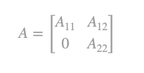
The canonical form of matrix A, shows that the production system using technique [A,l] produces both basic and non-basic commodities. Let the system produce m basic commodities and n-m non-basic commodities1. As a result, A11 is a square indecomposable mxm matrix and A22 is a square indecomposable (n-m)x(n-m) matrix. We further assume, that since rank(A)=n, rank (A11)=m and rank (A22)=n-m hold, then A11 and A22 are nonsingular. Let also matrix A12 be indecomposable2.
The previous assumption, that technique [A,l] is productive, implies that: 
of of matrix . It also holds for

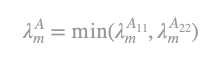
and

(the maximum eigenvalues of matrices, A11 and A22) respectively:
Thus, it holds:
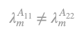
We further assume that:
The following definitions are implied:
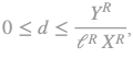
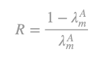
a) r is the given production system’s and its subsystems’ uniform profit rate. b) R represents the maximum profit rate of the given production system, which corresponds to a zero-nominal wage, w. c) R ̅ is the value of R, which assures positive or at least semi-positive prices for all commodities that [A,l,X] produces. It is obvious that R ̅ is the smallest positive value of R. Let wages be paid post factum. The following relationship describes commodity prices, p: 
Replacing w with zero in (1) it follows:
From (2) it follows that:
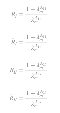
We furthermore denote:
- RI (RII) the maximum profit rate of subsystem I (II).
- R ̅I (R ̅II) the value of RI (RII), which ensures positive prices pI (pII) for all commodities that subsystem I (II) produces as net product. We obtain for the prices of the two subsystems: 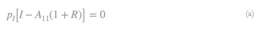
And
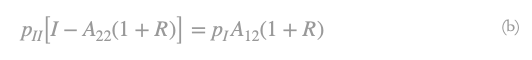
From (a) and (b) we can deduce that:
What has been said about the given production system [A,l,X], also holds for any other production system [A,l,V], which uses production technique [A,l] (Stamatis, 1998).
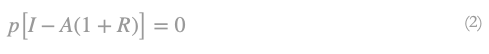
From equation (2) it follows that, to have a solution different than the trivial one ( p=0) it must hold: rank[I-A(1+R)]
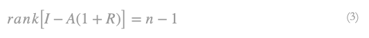
When (3) holds, then the inverse of [I-A(1+r)] also exists for r,0≤r≤R ̅ and consequently w,0≤w≤wmax. From (1) we obtain:
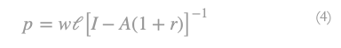
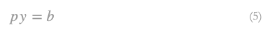
Equation (4) fully determines the price vector and up to a scalar for an exogenously given , or for an exogenously given w. It is concluded that prices cannot be fully determined for an exogenously given r, or w. To fully determine prices and obtain the w-r relation, it is mandatory to normalize prices first. The arbitrary determination of the price of a commodity or of a basket of commodities is called price normalization (Stamatis, 1991). The price normalization is accomplished by equating the price of a commodity or the price of a basket of commodities to a constant positive quantity of a homogeneous extensive thing. This equation is called normalization equation, the commodity mentioned above (basket of commodities) normalization commodity/ies and the positive quantity of a homogeneous extensive thing is called fictitious money. Let the normalization commodity be y, y ≥ 0. Let also the price of this commodity be equal to b units of fictitious money, or otherwise b units of that homogeneous extensive thing. Then the normalization equation is:
When we multiply equation (4) with (5) we can obtain the w-r relation, which is:
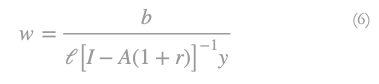
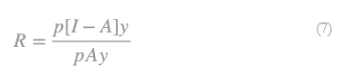
For r,0≤r≤R ̅ and w,0≤w≤wmax. It also holds for w=0:
We can derive from production system [A,l,X], its’ part [A*,l*,X*], which is called the normalization subsystem, by eliminating from vectors x,y,l (and thus we obtain x*, y*, l*), those components, related with the goods that only produce the given (and not the normal subsystem) system of production. Accordingly, we can derive from nxn matrix A, the kxk matrix A*, by eliminating rows and columns related to the above commodities. Correspondingly we can also derive p* from p.
Let R* be the maximum profit rate of the normalization subsystem and R ̅* the respective profit rate, which guarantees positive process. Based on the above, we can derive two distinguished types of normalization: If the normalization commodity consists only of basic commodities, it follows that: A*=A11. Then it holds 
And moreover
As R* we define the maximum profit rate of the normalization subsystem and as R¯* the profit rate which guarantees positive process.
On the other hand, if the normalization commodity consists of both basic and non-basic commodities, it follows that: A* = A . Then it holds (Stamatis G. 1998 p.12): 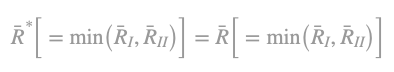
Therefore, it is possible to have:
for a normalization commodity consisting only of basic commodities and
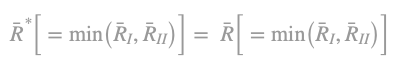
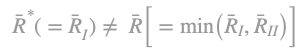
for a normalization commodity consisting of both basic and non-basic commodities.
Based on the above, we can substitute relations (1), (2), (3), (4) , (5) , (6) , (7) with (1a), (2a), (3a) , (4a) , (5a) , (6a) , (7a) respectively: 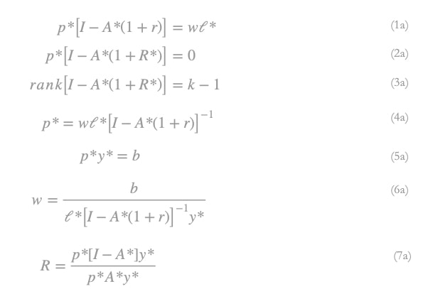
We have seen that the maximum profit rate of the normalization subsystem may be different from the maximum profit rate of the given subsystem. This implies that the position of the w-r curve may change with price normalization.
When normalization commodity changes, the normalization subsystem, that produces the normalization commodity, as its net product, also changes. With the normalization subsystem changing the obtained w-r relation also changes. The w-r relation does not belong to the technique [A, I] but to the normalization subsystem [A*, I*, X*], instead. It is possible in other words to have as many w-r relations as the correspondent normalization subsystems.
Consequently, when normalization commodity changes, the normalization subsystem and the correspondent w-r relation3 also change. The place (the maximum profit rate, the labor productivity in price terms), the slope4 and the shape (the second derivative of the w-r relation) of the w-r curve also change. Based on that, the phenomena of switching and reswitching may appear or disappear. Moreover, the choice, the order and the ranking of production techniques are generally impossible, since there are no production techniques to choose, order or rank but normalization subsystems instead. The only possible case for an unambiguous choice, order and ranking of techniques s is when the w-r relation is linear. The w-r relationship is linear, when prices were first normalized with Sraffa΄s (1960), Miayo΄s (1977) or Vassilakis’ (1983) standard commodity. Another example of a unambiguous choice is when the surplus product and the material inputs have the same composition. This is possible in Charassofian systems and of course in corn economies a la Ricardo (Manoudakis, 2010). Actually Ricardo was the first, who solved the above problem using the corn model.
The corn system
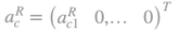
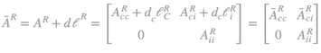
The Ricardian corn system consists of n production sectors5. The first sector produces corn (c), using only corn as a material input. The n-1 other sectors (i) produce other commodities by using corn and the remaining other n-1 commodities. The system uses a linear production function and each production process produces a single commodity. The profit rate r,r>0, is uniform and the real wages are represented by the vector d,d=(dc 0). The form of real wages vector implies that real wage consists only of corn6. Therefore, the given production technique is a closed a la Leontief model. Obviously, it is assumed that production technique is productive7 and the production system is viable. The Ricardian production system can be described by the triplet [AR,lR, XR], where b>lR,lR>0 the labor inputs entering directly in the production process of a unit of commodity, and XR, XR≥0, the gross product of the Ricardian system. Let matrix AR,AR≥0 be the Ricardian material input matrix, with the following canonical form: 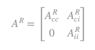

is the quantity of the other n-1 commodities (i) entering directly in the production process of a unit these commodities9 (i). The dlR matrix of real wages per unit of produced commodity is equal to:
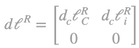
It is obvious that since real wages consist only of corn, material inputs and the real wages have the same composition. Accordingly we can define matrix
which represents the input matrix of means of production and wage commodities per unit of produced commodity10. In the Ricardian corn model not only, real wages but profit rate as well can be expressed in corn terms. It follows, thus, that real wages (which are included in the material inputs) and profits have the same composition. In terms of modern economics, the Ricardian corn model is decomposed into two subsystems: the reproductive one, which produces corn, and the non-reproductive one, which produces all other n-1 non-reproductive commodities. Profit rate is therefore determined as the ratio of the net product of the corn system and the sum of material (in corn) and labor inputs. Competition among production process, leads to the dominance of profit rate in the production process of corn over the production processes of all other n-1 commodities and thus to be uniform. The abovementioned common composition of profits and real wages entails a price-independent profit rate determination. The corn economy therefore, has the properties of a one-good economy.
Let the gross product, of the reproductive subsystem be equal to a unit of corn. Therefore, the net product is equal to 
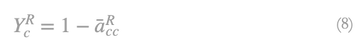
consists also of labor inputs. In that case net product is also the surplus product of this economy. Equation (9) represents the price system of the corn economy
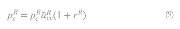
From (9) is implied:
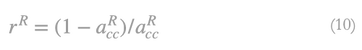
From equation (9) it is obvious that profit rate is independent from price normalization, while from equation (10) is implied that profit rate is the ratio of two magnitudes, sharing the same composition, namely the surplus product and the material inputs. Given equations (9) and (10), prices of the non-reproductive products can also be determined11. We have seen, how ingeniously had Ricardo solved the profit determination problem, independently of prices and how he had made the unambiguous choice of techniques possible.
Concluding remarksWe have seen how price normalization changes the w-r relation in decomposable production systems. The reason is quite simple: we cannot fully determine the prices without first normalizing the prices. Price normalization can change the dimensions of the production system, converting the production technique used by the given system, into a normalization subsystem. The existence of multiple subsystems can change the maximum profit rate of the normalization subsystem. Therefore, there is no need for the profit rate of the given production technique, and the profit rate of the normalization subsystem to coincide. Price normalization also changes the slope of the w-r curve (in other words the capital intensity of the normalization subsystem in price terms). The latter also changes the shape of the w-r curve. It is well known that w-r curve serves as the basis, for applying the profit maximization criterion. This criterion has been for decades a popular tool for economists to choose among techniques although, as has been shown above, they do not actually choose between techniques, but among the normalization subsystems. The fact that prices depend on the rate of profit and the rate of profit depends on the normalization of prices makes it impossible to choose techniques in the general case. Ricardo approximately 150 years before the so-called Cambridge Controversy, has found a way to overcome the above difficulties, although even then he was not aware of it. Having identified the vicious circle of prices, profit rate and wage determination, he had ingeniously introduced the framework of "common composition". He knew, in determining prices, an income distribution variable (he choose real wages) should first be determined exogenously. Real wages and moreover labor itself consisted as one commodity (re)produced in the Ricardian production system. Considered that, real wage is determined based technological attributes only, independently of price normalization and profit rate. As a result, the material inputs, the net product (at the same time the surplus product) and the real wages had the same composition. Given all the above assumptions and conclusions, he managed to determine profit rate independently of price normalization. In the corn model price normalization was not mandatory for determining the profit rate. Profit rate could easily be determined for each positive vector of prices. The above determination made it possible to choose unambiguously among techniques, since in corn models all the normalization subsystems coincide with the given production technique. So 150 years before Sraffa, Ricardo introduced a well-defined method of determining the profit rate.
1. It is obvious that 1≤m≤n
2. In other words, the given production system is decomposed into two subsystems: subsystem I which produces only basic commodities and subsystem II which produces basic and non-basic commodities. 3. The w-r relation can be re-written as: 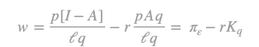
where πε≡(p[I-A])/lq is the productivity of labor in the normalization subsystem and Kq≡pAq/lq is the capital intensity, and the slope of the w-r curve, of the normalization subsystem.
4. The slope of the w-r curve is equal to 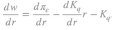
It holds for

In the special case that the w-r is linear then it holds

otherwise it holds

5. In the Ricardian framework there are three solid social classes: i) landowners own the land, which they rent, ii) capitalists who possess the capital, by which they buy labor power and organize the production and iii) workers who sell their labor force to the capitalists. In our model we have assumed that land can be extended indefinitely, and therefore, we have included it in the material input matrix. We further assume that all land pieces are equally productive. Consequently, all landowners receive the same rent. The above assumptions do not affect the results our analysis, but simplify it instead, since in Ricardo all the income variables are expressed in corn terms. In Pasinetti (1980) the analysis is more complex since the production of corn is referred to decreasing returns to scale and the luxurious product (gold) is subjected to constant returns to scale.
10. It is obvious that corn is a reproductive commodity and the other commodities are non-reproductive commodities. Thus Ricardo’s corn system can be represented in a canonical form with a decomposable non-singular matrix.
11. It holds for the price of the non-reproductive system: 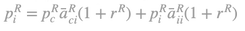
|